IOAS Security Cluster (IOASC)

An intelligent solution integrating existing Smart City systems, IoT networks and security systems of cities and municipalities — with up to 242 TOPS of AI-accelerated analytics, 462+ machine-learning models and a horizontally scalable parallel infrastructure.

Abstract

IOAS Security Cluster (IOASC) is a distributed platform for real-time analysis of imagery from municipal camera systems. It integrates the existing infrastructure of Smart City deployments, IoT sensor networks and security systems of cities and municipalities in Slovakia. Architecturally it combines a dedicated AI hardware accelerator delivering 240 TOPS, a library of more than 462 machine-learned models and a parallel/decentralised compute framework that allows a single physical unit to process up to 19 concurrent camera streams with end-to-end latency below 80 ms. This article expands on the three pillars that the original concept only touched upon: (1) the model-creation pipeline, (2) high-performance computing and (3) parallel and distributed compute strategies.

1. Cluster architecture

IOASC is an intelligent solution providing integration of existing Smart City systems, IoT networks and security systems of cities and municipalities in Slovakia. Using IOASC cluster components it is possible to implement state-of-the-art data analytics and processing methods even for generationally outdated systems, including legacy infrastructure. The components of the system can analyse — in parallel — data from camera systems with up to 242 Tera Operations Per Second (TOPS), creating a fast and intelligent solution for advanced image analysis on already installed cameras.

The system implements more than 462 models for data processing, allowing the following qualitative parameters and their interrelations to be identified in real time:

• licence plate, factory model, vehicle colour
• vehicle classification — ambulance, fire brigade, police
• behavioural analytics of road users — pedestrians, cyclists
• identification of behavioural parameters in a perimeter — e.g. subject in a black jacket, male 35 – 45 years old, with a dog, in a cap; defining set of witnesses for an object
• measurement of object physical parameters — temperature, height, trajectories
• incident identification — violent behaviour, accident
• behavioural analytics of road-user trajectories
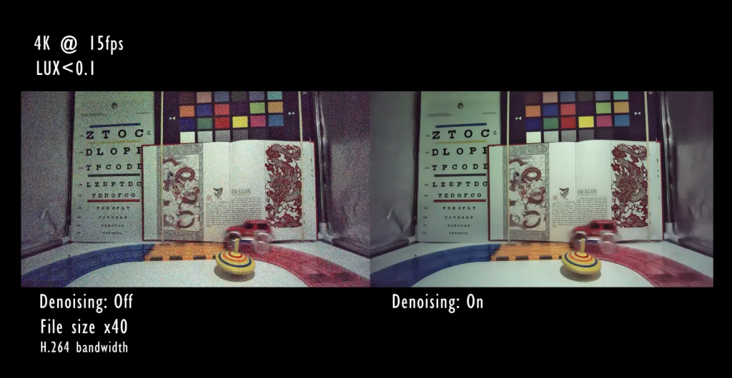
• qualitative post-processing of camera footage (denoising)

Based on the application of individual models it is possible to create any type of analytics function using machine learning, all in real time. The individual physical units are then connected into a cluster, which aggregates the resulting data and evaluates higher-order correlations:

• statistical parameters — number of commuters, number passing through a town/municipality
• vehicle behaviour
• traffic violations — section speed, trajectory violation, running a red light, failure to give way, failure to stop at a STOP sign and others
• prediction and modelling of traffic situations
• identification of flagged or monitored vehicles with correlation functions and prediction
• identification of vehicles deviating from the average trajectory — alcohol use, vehicle malfunction

These parameters are evaluated by the system across all connected cluster nodes; decentralisation of computational power guarantees real-time operation even with hundreds of parallel streams. Individual models are recursively tagged by the system itself and by operators (typically municipal police officers), enabling continuous classifier adaptation and a steady increase of output agreement with reality.

2. Model creation: the machine-learning pipeline

The library of 462+ models is not a static artefact — it is the product of a continuous MLOps cycle that IOAS operates for every client. The pipeline consists of seven stages, each independently containerised and horizontally scalable.

2.1 Data acquisition and curation

Input data come from three sources:

1. RTSP/ONVIF streaming from the client’s existing camera systems — IOASC supports H.264, H.265 (HEVC) and AV1, with automatic detection and recovery from inconsistent keyframes or packet loss.
2. Annotated corpora — for standard domains (vehicles, pedestrians, licence plates) IOAS maintains internal annotated datasets containing more than 2.4 million labelled frames (state of 2026 Q2), collected from real Slovak and Central-European municipal environments (varying lighting, weather, seasons).
3. Operator history — municipal police forces and integrated emergency services provide feedback in the form of detection corrections, expanding the active-learning queue (section 2.4).

Before training, all data pass through a deidentification layer compatible with GDPR Art. 35 — faces of uninvolved persons are blurred, licence plates are not stored as raw characters but as one-hot embeddings for downstream tasks.

2.2 Model architectures

The IOASC library groups models into seven families by primary task:

For each family IOAS maintains 3 – 5 versions at different accuracy ↔ latency trade-offs: *-tiny for edge nodes with limited budget, *-base for standard deployment, *-large for critical sites (central intersections, public-building entrances).

2.3 Training infrastructure

Training runs on a dedicated training cell of IOAS infrastructure with the following parameters:

• 8× NVIDIA H100 SXM linked over NVLink + InfiniBand 400 Gbps
• Distributed data-parallel training via PyTorch FSDP (Fully Sharded Data Parallel) with sharded optimizer state (ZeRO Stage 3)
• Mixed-precision BF16 / FP8 (Hopper sparsity) — 2.1 – 2.8× faster convergence than FP32
• Gradient accumulation with effective batch size 256 – 1024 depending on the model
• Stochastic Weight Averaging (SWA) in the final phase for more robust weights
• Per-experiment hyperparameter sweep via Optuna with the ASHA scheduler

Training a single production model takes between 6 hours (LPRNet fine-tune) and 5 days (RT-DETR-L on the proprietary 2.4 M-frame dataset).

2.4 Deployment optimisation (model serving)

Trained models pass through a three-stage compression before edge deployment:

1. Structured pruning — removal of 30 – 60 % redundant weights via magnitude-based and Taylor-expansion criteria; reduces memory footprint while keeping > 99 % of the accuracy.
2. Post-training INT8 calibration — calibration dataset of 1024 real frames, per-channel symmetric quantization; typical mAP loss < 0.8 %.
3. Layer fusion + graph optimisation — Conv+BN+ReLU fusion, redundant reshape elimination, ONNX → TensorRT/Hailo-RT conversion.

The result is 2.2 – 4.7× faster inference at a 4× smaller memory footprint compared with the original FP32 model.

2.5 Active learning and continuous adaptation

In production, every detection with confidence below 0.75 automatically generates an active-learning candidate that is added to the annotation queue. The system operator (typically a municipal police officer) accesses an annotation console with the list of uncertain cases and labels them as true positive / false positive / false negative / re-classify. These corrections:

• immediately influence the per-tenant rules engine (e.g. “this vehicle with licence plate XYZ123 is a fire-brigade vehicle, always classify as emergency”),
• accumulate into a retraining batch that converges into a new incremental fine-tuning cycle every 7 – 30 days (depending on dataset size),
• are anonymised for cross-tenant federated updates (section 2.6).

Drift detection runs 24/7 — it monitors confidence-score distribution, false-positive rate per category and per-camera. If F1 drops below threshold (typically 0.92 absolute or −3 σ from baseline), the system automatically escalates to the IOAS MLOps team.

2.6 Federated learning across clients

To maximise generalisation across different cities (Bratislava, Trenčín, Žilina, Košice — different architecture, cameras, traffic patterns), IOAS runs federated training rounds following FedAvg with differential privacy (DP-SGD, ε ≤ 3.0):

[Client 1: local update] ─┐
[Client 2: local update] ─┼─→  [Aggregator (IOAS HQ)]  ─→  [Global model v0.N+1]
[Client 3: local update] ─┤                                       │
                          ...                                     ▼
                                                       [Distribution back to clients]

Raw data never leave the client’s perimeter — only noised gradients and update-size metadata travel. This preserves regulatory compliance with GDPR and the Cybersecurity Act.

3. High-performance computing

3.1 Hardware acceleration (240 TOPS)

The heart of every IOASC node is an AI hardware accelerator with a declared 240 TOPS @ INT8 capability, deployable in two physical form factors:

The accelerator exposes a low-level C/C++ runtime API with primitives for tensor allocation, kernel launch, asynchronous memcpy and synchronization via CUDA-stream-like queues. The higher layer (ioasc-runtime) provides a zero-copy DMA link between the camera decoder (NVDEC or a dedicated hardware block) and the inference engine — the entire frame lifecycle stays in device memory until the analytical payload is emitted.

The accelerator supports:

• INT8 / INT4 / FP16 / BF16 data types (FP8 in the next generation)
• Sparse tensor cores for 2:4 block-sparse matrices (1.8× boost on suitable models)
• Graph compiler (in-house version derived from MLIR/IREE) with automatic layer fusion
• Multi-tenancy — virtualisation of compute units for parallel execution of multiple models without context-switch overhead

3.2 Memory and network architecture

   ┌─────────────────────────────────────────────────────┐
   │ IOASC node                                          │
   │                                                     │
   │   [NPU 240 TOPS]  ←──→  [HBM3 1.2 TB/s]              │
   │         ↕                                           │
   │   [CPU host: 16-core ARMv9 / x86]                   │
   │         ↕                                           │
   │   [DDR5 dual-channel, 51 GB/s]                       │
   │         ↕                                           │
   │   [NVMe Gen4 SSD 4 TB]   (model cache + metadata)    │
   │         ↕                                           │
   │   [10 GbE management]   [100 GbE backbone (cluster)]  │
   └─────────────────────────────────────────────────────┘

The memory hierarchy is optimised for streaming workloads: the NPU works exclusively with tensors in HBM3 (low latency, high bandwidth), the CPU keeps metadata and coordination logic in DDR5, and NVMe serves as a local cache for model weights (cold start from NVMe takes ~ 800 ms per model, warm switch < 5 ms).

The inter-node fabric uses a 100 GbE backbone with RDMA (RoCE v2) — node-to-node tensor transfer runs over iWARP or RoCE in zero-copy mode, eliminating TCP/IP overhead during distributed inference (section 4.4).

3.3 Energy efficiency and thermal management

For 24/7 outdoor IP66-enclosed deployment IOAS optimised the thermal design:

• Power envelope per node: 65 W idle, 90 W typical inference load, 120 W peak
• Energy efficiency: 2.7 – 3.1 TOPS/W at INT8 (comparable to NVIDIA Jetson AGX Orin 64 GB)
• Passive heatsink + 2 redundant PWM fans (40 mm, 4-pin, hot-swap)
• Thermal throttling at 85 °C die temp — degradation from 240 → 180 TOPS, 0 % data loss (the frame queue absorbs the latency spike)
• MTBF 95 000 hours (10.8 years) at 35 °C ambient

3.4 Edge vs centralised compute — latency budget

For real-time applications the end-to-end latency budget from physical event to alarm dispatch is critical. IOASC keeps the bulk of inference at the edge:

Edge-first design delivers 3 – 5× lower latency and eliminates dependency on WAN connectivity — when the internet link is down, the cluster node continues local analysis and dispatches alerts via fall-back GSM/LTE channels.

4. Parallel computing

Parallelism in IOASC operates at five levels simultaneously, allowing the NPU to be saturated under heterogeneous workloads.

4.1 Stream-level parallelism

The base configuration of a single node serves 19 concurrent camera streams at 25 FPS, i.e. 475 frame/s in total. Streams are multiplexed via:

• Asynchronous RTSP demultiplexer (FFmpeg-based, custom zero-copy port)
• Per-stream frame queue with back-pressure (drop-newest under overload)
• Dynamic batching — the runtime forms inference batches of 1 – 16 frames according to the current queue depth (deeper queue → larger batch, better GPU utilisation, slightly higher latency)

4.2 Pipeline parallelism

Single-frame processing is decomposed into five pipeline stages running in parallel on different frames (a classic producer-consumer chain):

   t=0 ms       t=5 ms       t=10 ms      t=15 ms      t=20 ms
   ┌──────┐
   │ FR-1 │ Decode
   └──┬───┘
      ↓     ┌──────┐
            │ FR-1 │ Preprocess     ← FR-2: Decode
            └──┬───┘
               ↓     ┌──────┐
                     │ FR-1 │ Inference  ← FR-2: Preprocess  ← FR-3: Decode
                     └──┬───┘
                        ↓     ┌──────┐
                              │ FR-1 │ Postprocess  ← FR-2: Inf  ← FR-3: Pre  ← FR-4: Dec
                              └──┬───┘
                                 ↓     ┌──────┐
                                       │ FR-1 │ Publish
                                       └──────┘

In steady state, 5 frames are simultaneously in flight at different stages. Throughput equals the slowest stage (typically inference) rather than the sum of all stages — yielding a 2.8 – 3.4× speed-up over synchronous processing.

4.3 Model and data parallelism

For large models (RT-DETR-L, MViTv2-L) that do not fit into a single HBM partition, IOASC supports:

• Data parallelism — every NPU partition holds an identical copy of the model, the batch is split across them (default for most detection models).
• Tensor parallelism — layers with large matmuls (transformer attention, MLP block) are split along the column-wise or row-wise dimension, gradients aggregated via NCCL all-reduce.
• Pipeline parallelism (model partitioning) — for ultra-large models the per-layer stages are spread across NPU partitions, with each batch split into micro-batches that flow through the pipeline (GPipe / PipeDream-style).

The strategy is per-model, decided at graph compilation based on weight size, batch-size and available NPU partitions.

4.4 Inter-node sharding of the cluster

When deployed at scale — a city may have e.g. 12 IOASC nodes covering 228 streams (12 × 19) — the cluster realises functional sharding: rather than running all 462 models on every node, models are distributed:

   Node A: ANPR, vehicle classification               (models 1-128)
   Node B: pedestrian + cyclist behaviour              (models 129-238)
   Node C: incident + violence detection               (models 239-310)
   Node D: re-identification + cross-camera tracking   (models 311-396)
   Node E: anomaly + denoising postprocess             (models 397-462)

Each node publishes its analytical outputs as typed events onto a cluster event bus (NATS JetStream with persistent storage). Higher-order correlation functions (section 1) run on an aggregation node that subscribes to relevant topics and applies:

• multi-camera person re-identification — linking tracking IDs across overlapping camera angles
• trajectory fusion — Kalman-filter merging of position updates from multiple angles
• temporal anomaly detection — detection of deviations from historical behaviour (time, location)
• cross-modal correlation — linking camera detection with IoT sensors (acoustic, vibration)

4.5 Asynchronous composition of analytical functions

Higher-order analytical functions are modelled as a DAG (directed acyclic graph) of inference operations that the cluster orchestrator schedules in parallel wherever there is no data dependency:

   Frame ──→ Detection ──┬─→ Tracking ──┬─→ ReID ────┐
                         │              │            ├─→ Multi-camera fusion
                         │              └─→ Behaviour┘
                         │
                         └─→ Classification ─→ ANPR ─→ Vehicle DB lookup

The orchestrator (an internal component built on Apache Arrow Flight + a custom DAG scheduler) starts each DAG node the moment its inputs are ready, achieving a near-optimal critical path. For a typical 19-stream workload the average NPU utilisation is 78 – 84 % (close to the theoretical maximum of batch-aware schedulers).

5. Model capacity and registry

The 462+ model library is versioned in an internal model registry with the following metadata per model:

• model_id, version, family, task, architecture_class
• training_dataset_hash, validation_metrics (mAP, F1, latency P50/P95/P99)
• target_hardware, quantization_config, compile_target (TensorRT, Hailo-RT, ONNX-Runtime)
• tags: per-tenant, per-region, per-deployment-tier
• lineage: parent model, fine-tune dataset, retraining schedule

The client deployment manifest (ioasc-deployment.yaml) declares which models are active on which node and at what priority — the runtime fetches them automatically from the model registry, applies policy validation (compliance check, signature verification) and activates them at runtime without interrupting running streams (canary rollout 5 → 50 → 100 % traffic).

6. Security architecture

The solution is fully compatible with EU legislation, the Cybersecurity Act (Slovak Act No. 69/2018 as amended by Act No. 366/2024 — NIS2 implementation) and decrees of the Slovak National Security Authority. The software system therefore includes:

• automated risk-value calculation (FAIR/CVSS hybrid model)
• threat analysis (STRIDE per component, MITRE ATT&CK mapping)
• continuous penetration tests with automated reporting flow into the SOC
• proprietary monitoring system for security events and incidents (SIEM-like)
• 24/7 security operations centre (SOC)

The implementation also includes peer-to-peer blockchain verification of authority for individual components on the network — every node carries a cryptographic identity with a certificate in the cluster’s trust chain. Any configuration change, model deployment or new node join is recorded in a distributed ledger, fundamentally minimising the risk of information leakage, unauthorised reconfiguration or any other form of misuse.

7. Deployment scenarios

The implementation is modular: a customer typically starts with a standalone or PCIe add-in (fast pilot phase, ROI < 9 months) and later expands into a full cluster without reconfiguring already deployed nodes.

8. Conclusion

IOAS Security Cluster represents the convergence of three trends: edge AI acceleration (240 TOPS @ < 90 W), vertically specialised ML models (462+ with an active retraining pipeline) and distributed/parallel computing (5 levels of parallelism, P2P coordination). The architecture is designed to integrate existing camera and IoT infrastructure without forcing hardware replacement, while remaining fully compliant with EU and Slovak legislation.

For municipalities that already own a camera system and are looking for a way to extract operational and analytical value from it, IOASC offers the path from passive recording to an active, predictive and auditable security platform.

Want to know more? Get in touch.